Step 0: Segmenting a single cell from a volume image#
In order to remap a cell surface in u-Unwrap3D, the cell must be first segmented from the volumetric image to obtain a binary image. A surface mesh is then created from the binary image typically using the marching cubes algorithm.
This workbook walks through this process.
N.B: We illustrate the most basic way to segment a cell using an automatic binary thresholding method. This fundamentally assumes you have high signal-to-noise ratio image where the single cell is very well delineated from the background. Moreover it assumes the illumination is uniform and the cell is bright. Thus it is not generally applicable. If you have a better 3D segmentation method, please use that and only follow to see how to extract a surface mesh.
Warning concerning segmentation: In order to ensure the extracted mesh truly captures the surface, it is crucial to check in this step that the binary image is indeed capturing the whole cell such that the interior cell volume is ‘filled’. An easy check is to visualize a mid-section slice of the binary, and check the interior all has the equivalent of a binary 1. If this is not true, the cell will be ‘double-meshed’ and the extracted ‘surface’ actually represents the exterior shell. Whilst u-Unwrap3D can handle these imperfect surface meshes, they do affect quantification e.g. you will measure approximately twice larger surface area, and a very small cell volume.
1. Basic binary segmentation using Otsu thresholding#
We read in the volume image used in Fig.1 of the u-Unwrap3D paper and also create a savefolder to store the results of analysis.
import skimage.io as skio
import os
import numpy as np
import pylab as plt

import unwrap3D.Visualisation.volume_img as vol_img_viz # for creating a montage maximum projection
import unwrap3D.Utility_Functions.file_io as fio # for common IO functions

"""
Specifying image file location and parsing its name.
"""
imgfolder = '../../data/img'
imgfile = os.path.join(imgfolder, 'bleb_example.tif')

basefname = os.path.split(imgfile)[-1].split('.tif')[0] # get the filename with extension

"""
Initialise a save folder to store the important outputs for the result of the pipeline.
"""
savefolder = os.path.join('example_results',
                         basefname,
                         'step0_cell_segmentation')
fio.mkdir(savefolder) # auto generates the specified folder structure if doesn't currently exist.


"""
Read and display image
"""
# read the image using scikit-image
img = skio.imread(imgfile)

# utility function in u-Unwrap3D to generate a montage maximum projection of the 3 orthogonal views for display
img_proj = vol_img_viz.montage_vol_proj(img, np.max)


plt.figure()
plt.title('Montage maximum projection')
plt.imshow(img_proj, cmap='gray')
plt.grid('off')
plt.axis('off')
plt.savefig(os.path.join(savefolder,
                        basefname+'_max-proj_three.png'), dpi=300, bbox_inches='tight')
plt.show()
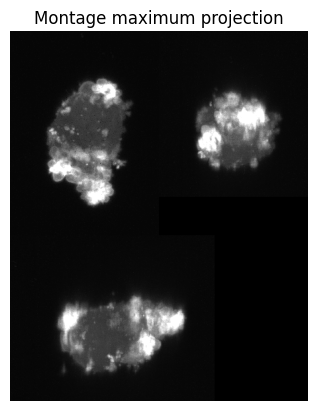
The image contains a single cell. The whole of the cell is brighter than the background. Moreover the signal-to-noise (SNR) ratio is excellent, with the cell well-delineated from the background. In this case, we can segment the single cell with an intensity threshold automatically determined by Otsu’s method from the scikit-image library (skimage.filters.threshold_otsu).
import unwrap3D.Segmentation.segmentation as segmentation # import the segmentation submodule which wraps the Otsu method
import scipy.ndimage as ndimage # use instead of scikit-image for faster morphological operations in 3D
import skimage.morphology as skmorph

# returns the binary and the auto determined threshold.
img_binary, img_binary_thresh = segmentation.segment_vol_thresh(img)
# erode by ball kernel radius = 1 to make a tighter binary
img_binary = ndimage.binary_erosion(img_binary,
                                    iterations=1,
                                    structure=skmorph.ball(1))
img_binary_proj = vol_img_viz.montage_vol_proj(img_binary, np.max)

plt.figure()
plt.title('Montage binary segmentation')
plt.imshow(img_binary_proj, cmap='gray')
plt.grid('off')
plt.axis('off')
plt.savefig(os.path.join(savefolder,
                         basefname+'_binary_three.png'), dpi=300, bbox_inches='tight')
plt.show()

"""
Save the binary out as a uint8 .tif
"""
skio.imsave(os.path.join(savefolder,
                         basefname+'_binary_seg.tif'),
            np.uint8(255*img_binary))
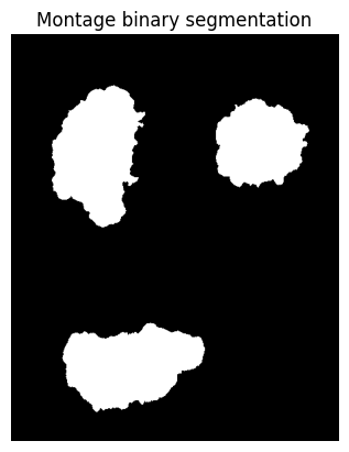
We see from the cross-section visualization of x-y, x-z and y-z views, that the segmentation captures the full cell, with the cell interior filled in (i.e. all white pixels). Therefore we move ahead to extract its surface using marching cubes.
2. Surface meshing the binary segmentation#
We mesh the binary segmentation (0 or 1 value) using marching cubes at an isovalue of 0.5. The triangles obtained from this are very heterogeneous. Ideally, in mesh analysis, triangles should be close to regular and equilateral. This is particularly important for later steps where we need to solve differential equations on the mesh. Therefore we apply remeshing on the marching cubes output.
u-Unwrap3D provides two isotropic remeshing algorithms: 1) pyacvd which uses voronoi clustering or 2) the incremental method of Botsch in CGAL based on splitting long edge lengths and collapsing short ones to obtain uniform triangles of a desired length.
We developed u-Unwrap3D initially using method 1 which does not work without requesting an output mesh with fewer vertices (typically at least < 0.5x starting number of vertices). We have since found that the Botsch method is more robust, computable for output mesh with more, same and less vertices, and it better preserves ‘sharp’ high curvature features. This is now our recommended method, and is used here.
import unwrap3D.Mesh.meshtools as meshtools # load in the meshtools submodule

img_binary_surf_mesh = meshtools.marching_cubes_mesh_binary(img_binary.transpose(2,1,0), # The transpose is to be consistent with ImageJ rendering and Matlab convention
                                                                presmooth=1., # applies a presmooth
                                                                contourlevel=.5,
                                                                remesh=True,
                                                                remesh_method='CGAL', # 'pyacvd' = method 1, 'CGAL' = method 2
                                                                remesh_samples=.5, # remeshing with a target #vertices. 0.5 = 50% of original vertex number
                                                                predecimate=False, # this applies quadric mesh simplication to remove very small edges before remeshing. This must be True if using method 1, 'pyacvd'
                                                                min_mesh_size=10000, # enforce at least this number of vertices.
                                                                upsamplemethod='inplane') # upsample the mesh if after the simplification and remeshing < min_mesh_size
"""
A quick way to check the genus is to get the euler number. The genus of the mesh is related to the euler number by
A genus-0 mesh should have euler number = 2
"""
print('Euler characteristic of mesh is: ', img_binary_surf_mesh.euler_number) #should be 2 if genus is 0

# we also provide a more comprehensive function for common mesh properties
mesh_property = meshtools.measure_props_trimesh(img_binary_surf_mesh, main_component=True, clean=True)

print(mesh_property) # note: if we have a proper surface mesh, 'volume'=True, Technically the mesh should also be 'watertight' but this is too strict a condition and often doesn't hold true for meshes of complex cell surface morphologies obtained from cell segmentation.

# we also provide a function to check triangle quality.
triangle_property = meshtools.measure_triangle_props(img_binary_surf_mesh, clean=True)
print(triangle_property)
Euler characteristic of mesh is:  2
{'convex': False, 'volume': True, 'watertight': True, 'orientability': True, 'euler_number': 2, 'genus': 0.0}
{'min_angle': 26.72508986342643, 'avg_angle': 60.0, 'max_angle': 120.22838447281411, 'std_dev_angle': 7.929529219591057, 'min_quality': 0.45590905439225127, 'avg_quality': 0.9721451710158225, 'max_quality': 0.9999995344888766, 'quality': array([0.94127854, 0.96283626, 0.98680869, ..., 0.99574797, 0.97367502,
       0.9432703 ]), 'angles': array([[0.78888048, 1.09433584, 1.25837634],
       [1.18150819, 0.83259891, 1.12748555],
       [0.9941968 , 0.9659957 , 1.18140015],
       ...,
       [0.97521725, 1.10067972, 1.06569568],
       [1.0237358 , 1.22173832, 0.89611853],
       [1.29700637, 1.02794175, 0.81664453]])}
3. Measuring the mean curvature of the surface, \((H(S(x,y,z)))\) and coloring on the surface mesh#
There are many ways to determine the mean curvature of the surface with different pros and cons.
From surface mesh
Measuring surface mean curvature typically involves fitting a local plane to neighborhood vertices of a surface mesh. see: unwrap3D.Mesh.meshtools.compute_mean_curvature. If the surface mesh has topological errors, e.g. containing holes, this measurement is not accurate. It can also be subject to the quality of the triangle faces and choice of neighborhood radius.
From binary segmentation
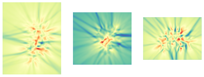
We find it easier and more accurate for downstream quantification to measure curvature from the continuous definition of mean curvature, \(H\) using the binary segmentation whereby we can easily apply morphological operations like dilation and hole-filling to fix small mesh errors.
where \(\hat{n}\) is the unit surface normal vector, and also the gradient of the signed distance function \(\Phi\) of the binary segmentation.
The curvature at the surface is then obtained by interpolating at the surface mesh vertices.
This is however typically slower.
import unwrap3D.Mesh.meshtools as meshtools

# compute the continuous mean curvature definition and smooth slightly with a Gaussian of sigma=3.
surf_H, (H_binary, H_sdf_vol_normal, H_sdf_vol) = meshtools.compute_mean_curvature_from_binary(img_binary_surf_mesh,
                                                                                    img_binary.transpose(2,1,0),
                                                                                    smooth_gradient=3, # adjusts smoothing, plays similar role to neighborhood radius in mesh method
                                                                                    eps=1e-12,
                                                                                    invert_H=False, # set True if you want positive values to correspond to positive curvature on the surface like blebs and binary is not transposed, otherwise set False.
                                                                                    return_H_img=True) # set return_H_img to be True, if

plt.figure(figsize=(10,10))
plt.subplot(131)
plt.imshow(np.nanmean(H_binary,axis=0), cmap='Spectral_r'); plt.grid('off'); plt.axis('off')
plt.subplot(132)
plt.imshow(np.nanmean(H_binary,axis=1), cmap='Spectral_r'); plt.grid('off'); plt.axis('off')
plt.subplot(133)
plt.imshow(np.nanmean(H_binary,axis=2), cmap='Spectral_r'); plt.grid('off'); plt.axis('off')
plt.show()
import unwrap3D.Image_Functions.image as image_fn # for common image processing functions
import unwrap3D.Visualisation.colors as vol_colors # this is for colormapping any np.array using a color palette
from matplotlib import cm # this is for specifying a matplotlib color palette


"""
We map the curvature values to a colorscheme for display. To set the scale, we use the voxel size to convert to metric units of $\mu m^{-1}$
"""
# we generate colors from the mean curvature
voxel_size = 0.104 #um
surf_H_colors = vol_colors.get_colors(surf_H/voxel_size, # 0.104 is the voxel resolution -> this converts to um^-1
                                      colormap=cm.Spectral_r,
                                      vmin=-1.,
                                      vmax=1.) # colormap H with lower and upper limit of -1, 1 um^-1.

# set the vertex colors to the computed mean curvature color
img_binary_surf_mesh.visual.vertex_colors = np.uint8(255*surf_H_colors[...,:3])

# save the mesh for viewing in an external program such as meshlab which offers much better rendering capabilities
tmp = img_binary_surf_mesh.export(os.path.join(savefolder, 'curvature_binary_mesh_'+basefname+'.obj')) # tmp is used to prevent printing to screen.
The saved surface mesh is in .obj format. These are best viewed in a dedicated mesh viewer such as meshlab, or chimerax which are opensource, free and cross-platform.
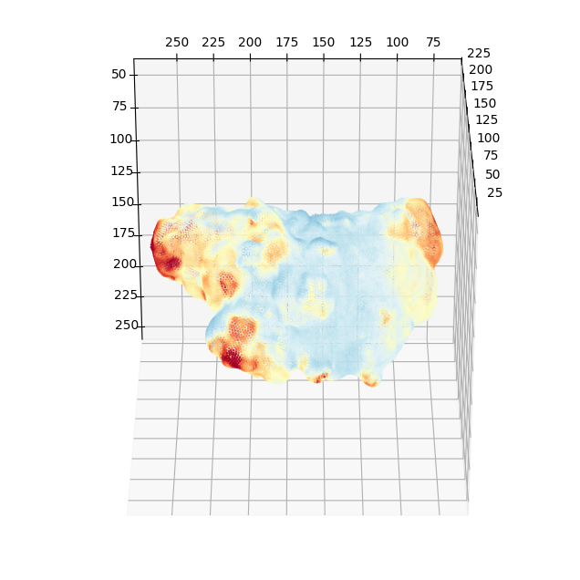
Within python, we can get an idea without installing more specialized libraries such as vedo by 3D scatter plotting and coloring the mesh vertices with matplotlib.
import unwrap3D.Visualisation.plotting as plotting # we import this so we can make x,y,z axes be plotted in equal proportions.

fig = plt.figure(figsize=(8,8))
ax = fig.add_subplot(projection='3d')
ax.scatter(img_binary_surf_mesh.vertices[...,2],
           img_binary_surf_mesh.vertices[...,1],
           img_binary_surf_mesh.vertices[...,0],
           s=1,
           c=surf_H/voxel_size,
           cmap='Spectral_r',
           vmin=-1,
           vmax=1)
ax.view_init(-60, 180)
plotting.set_axes_equal(ax)
plt.show()
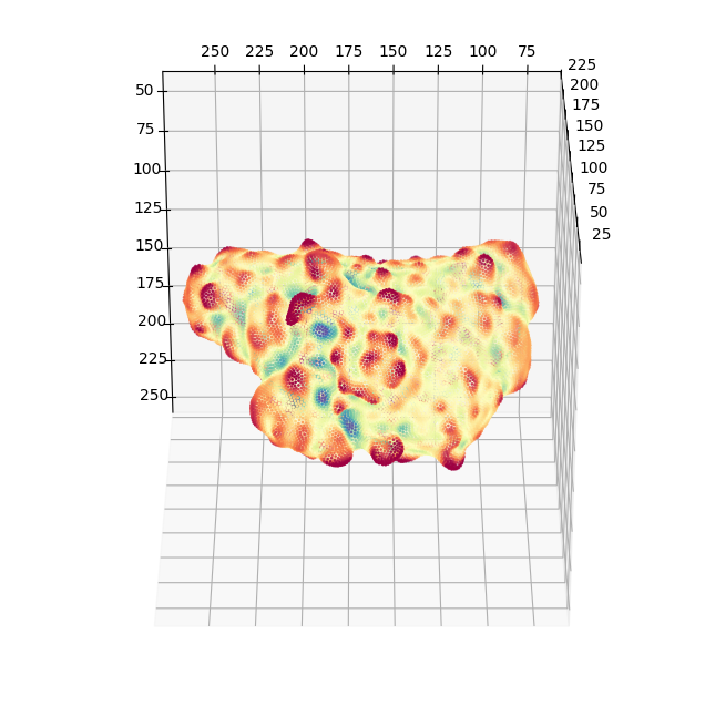
4. Map surface proximal membrane signals by traversing along the gradient of a distance transform into the cell#
We can use active contour conformalized mean curvature flow, (see the u-Unwrap3D paper) to traverse into the cell and sample the image intensity at designed step sizes \(\alpha\) along the gradient of a signed distance function. We can then average the sampled intensity and map this onto the cell surface. We do this for our cell up to 1 \(\mu m\) depth. Our image has an isotropic voxel resolution of 0.104 \(\mu m\). We sample this depth in steps of 0.5 voxels. This equates to a total of 1./(0.104*0.5) steps rounded down to the nearest integer.
n_samples = 1./ voxel_size # total number of steps
stepsize = 0.5 # voxels

# flip the mesh vertex coordinates so that it aligns with the volume size
img_binary_surf_mesh.vertices = img_binary_surf_mesh.vertices[:,::-1].copy()

# run the active contour cMCF to get the coordinates at different depths into the cell according to the external image gradient given by the gradient of the signed distance function.
v_depth = meshtools.parametric_mesh_constant_img_flow(img_binary_surf_mesh,
                                                      external_img_gradient = H_sdf_vol_normal.transpose(1,2,3,0),
                                                      niters=int(n_samples/stepsize),
                                                      deltaL=5e-5, # delta which controls the stiffness of the mesh
                                                      step_size=stepsize,
                                                      method='implicit', # this specifies the cMCF solver.
                                                      conformalize=True) # ensure we use the cMCF Laplacian

# we can check the size of the array
print(v_depth.shape)

# we can plot the trajectory with matplotlib
100%|██████████| 19/19 [00:05<00:00, 3.30it/s]
(23864, 3, 20)
Implementation Warning Note:
We typically use the signed distance function given by the Euclidean distance transform (EDT) as illustrated above to deform the mesh and sample the intensities, as it is fast to compute and memory-efficient. However, when sampling thin, narrow, and long protrusions. The result of the EDT will look ‘blocky’. In these cases, it is more optimal to compute the signed distance function given by solving the Poisson equation (see: unwrap3D.Segmentation.segmentation.poisson_dist_tform_3D). However, our current implementation uses an exact LU solver which is slow and will likely memory error. We recommend computing the distance transform on the isotropically downsampled binary segmentation (e.g. 1/8th), then resizing the result to the original size. This is valid because the distance transform is smooth.
# get the intensities at the sampled depth coordinates.
v_depth_I = image_fn.map_intensity_interp3(v_depth.transpose(0,2,1).reshape(-1,3),
                                            img.shape,
                                            I_ref=img)
v_depth_I = v_depth_I.reshape(-1,v_depth.shape[-1]) # matrix reshaping into a nicer shape.

# postprocess to check the total distance from the surface does not exceed the desired and replace any nans.
dist_v_depth0 = np.linalg.norm(v_depth - v_depth[...,0][...,None], axis=1)
valid_I = dist_v_depth0<=n_samples
v_depth_I[valid_I == 0 ] = np.nan # replace with nans


# compute the mean sampled intensity which will be taken as the surface intensity.
surf_intensity_img_raw = np.nanmean(v_depth_I, axis=1)
surf_intensity_img_raw[np.isnan(surf_intensity_img_raw)] = 0

# for visualization, we find the intensity range to be more pleasing if clipped to between the 1st and 99th percentile.
I_min = np.percentile(surf_intensity_img_raw,1)
I_max = np.percentile(surf_intensity_img_raw,99)

surf_intensity_img_raw_colors = vol_colors.get_colors(surf_intensity_img_raw,
                                                      colormap=cm.RdYlBu_r,
                                                      vmin=I_min,
                                                      vmax=I_max)
# create a new surface mesh, now with the PI3K molecular signal colors.
img_binary_surf_mesh_colors = meshtools.create_mesh(vertices=img_binary_surf_mesh.vertices[:,::-1],
                                                  faces=img_binary_surf_mesh.faces,
                                                  vertex_colors=np.uint8(255*surf_intensity_img_raw_colors[...,:3]))
tmp = img_binary_surf_mesh_colors.export(os.path.join(savefolder,
                                                'PI3K_binary_mesh_'+basefname+'.obj')) # tmp is used to prevent printing to screen.


# again we can quickly view the coloring in matplotlib
fig = plt.figure(figsize=(8,8))
ax = fig.add_subplot(projection='3d')
ax.scatter(img_binary_surf_mesh_colors.vertices[...,2],
           img_binary_surf_mesh_colors.vertices[...,1],
           img_binary_surf_mesh_colors.vertices[...,0],
           s=1,
           c=surf_intensity_img_raw,
           cmap='RdYlBu_r',
           vmin=-I_min,
           vmax=I_max)
ax.view_init(-60, 180)
plotting.set_axes_equal(ax)
plt.show()


# finally we will save the actual numerical values of the surface curvature and intensity to avoid recomputation to use for other steps of the pipeline
import scipy.io as spio # we save in .mat, this will allow matlab users to use the output if desired
spio.savemat(os.path.join(savefolder,
                          basefname+'_surface_curvature_intensity_stats.mat'),
            {'surf_H': surf_H,
             'surf_intensity' : surf_intensity_img_raw})